An LTAO reconstructor for KAPA
This tutorial builds a laser tomography reconstructor for KAPA, the Keck All-sky Precision Adaptive optics system: four sodium laser guide stars on a 7.6″ asterism, a 20×20 Shack–Hartmann per guide star, and a 21×21 actuator deformable mirror.
By the end you will have produced a single matrix that maps 2432 raw slopes to DM commands.
Setup
git clone https://github.com/KeckObservatory/pyTomoAO.git
cd pyTomoAO
pip install .
import numpy as np
from pyTomoAO import example_config
from pyTomoAO.reconstructor import tomographicReconstructor
Step 1 — Load the configuration
reconstructor = tomographicReconstructor(example_config("kapa"))
Loading parses and validates all five parameter sections. Print them to confirm the geometry is what you expect:
print(reconstructor.lgsAsterismParams)
print(reconstructor.lgsWfsParams)
The important numbers for what follows:
nLGS = 4guide stars, so four WFS channels.nValidSubap = 304valid subapertures per WFS, hence 608 slopes per channel and 2432 slopes in total.A seven-layer atmosphere observed at 30° zenith angle.
Step 2 — Build the model-based reconstructor
R = reconstructor.build_reconstructor()
print(f"Reconstructor matrix shape: {R.shape}")
This computes the slope covariance across all four sensors, the phase-to-slope cross-covariance for the on-axis optimisation direction, and inverts the system. On a CPU this takes a while for a system this size; with CuPy installed the GPU kernels are used automatically (see GPU acceleration).
To trade noise propagation against fidelity, pass a different regularisation weight:
R = reconstructor.build_reconstructor(alpha=10) # default
Step 3 — Reconstruct a wavefront
Build a slope vector to test with. Here is a pure tip-tilt signal, identical on all four sensors — negative X slopes, positive Y slopes:
slopes = np.ones(608)
slopes[:304] = -1
slopes = np.tile(slopes, 4)      # 2432 slopes total
wavefront = reconstructor.reconstruct_wavefront(slopes)
fig = reconstructor.visualize_reconstruction(slopes)
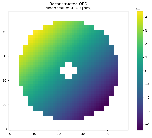
Reconstructed optical path difference. Points outside the pupil mask are NaN.
A tilt in, a tilt out — if you see structure that does not match your input, the slope ordering is the first thing to check.
If you have a reference wavefront (from a simulation, say), pass it in for a three-panel comparison including the residual:
fig = reconstructor.visualize_reconstruction(slopes, reference_wavefront=reference)
Step 4 — Add the fitting step
The model-based reconstructor outputs phase. To get DM commands, assemble it with the influence function fit:
FR = reconstructor.assemble_reconstructor_and_fitting(
    nChannels=4,
    slopesOrder="simu",
    scalingFactor=1.5e7,
)
print(f"Reconstructor + fitting matrix shape: {FR.shape}")
slopesOrder="simu" matches the slope vector built above — all X slopes then all Y slopes
per channel. For slopes coming from the Keck real-time controller, which interleaves X and
Y per subaperture, use slopesOrder="keck" instead.
KAPA’s central actuator is not controlled, so mask it out:
reconstructor.mask_DM_actuators(174)
FR = reconstructor.FR
fig = reconstructor.visualize_commands(slopes)
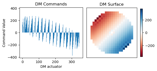
DM commands derived from the reconstructed phase.
Step 5 — Apply it
FR is now everything the real-time path needs:
commands = FR @ slopes
Save it for your controller:
np.save("kapa_FR.npy", FR)
Variant — an IM-based reconstructor
If you have measured an interaction matrix for KAPA, block diagonal with one block per WFS, you can bypass the influence function model entirely:
IM = np.load("kapa_IM.npy")

R = reconstructor.build_reconstructor(IM)
print(f"Reconstructor matrix shape: {R.shape}")

fig = reconstructor.visualize_commands(slopes)
There is no assembly step here — the output of R @ slopes is already in command space.
Note that reconstruct_wavefront and assemble_reconstructor_and_fitting will raise
ValueError on an IM-based reconstructor, since there is no intermediate phase estimate.
Single-channel operation
To use the same configuration with only one wavefront sensor — during single-conjugate
testing, for instance — set nChannels=1:
reconstructor = tomographicReconstructor(
    example_config("kapa-single-channel")
)
reconstructor.build_reconstructor()
FR = reconstructor.assemble_reconstructor_and_fitting(nChannels=1, slopesOrder="simu")
The reconstructor is truncated to the first sensor’s subapertures, so the expected slope vector is 608 elements rather than 2432.
Where to go next
Configuration reference — adapt the configuration to your own system.
DM fitting — calibrate
scalingFactorand DM orientation.API reference — the full API surface.